I had wanted to build my own AI for a while. I had used different types of AI at work (symbolic NLU, RAG, OCR, STT, TTS, agents, and LLMs), but I never truly understood what was happening behind the scenes.

My brother studied this field, so I asked him to guide me through building one.

We chose a very serious and important problem: distinguishing dogs from muffins.

Apparently, it’s a classic exercise taught in engineering schools, and a dataset already exists for it.

My goal was to satisfy my curiosity about how models are built, learn some of the vocabulary, and understand the environment and tools required for this kind of project.

For this project, we will use machine learning, more specifically, deep learning. Since we have labeled examples of dogs and muffins, this is a supervised learning task. To solve it, we will build a Convolutional Neural Network (CNN).

Vocabulary

To understand each other, we first needed a little of AI vocabulary. I’ll go through what we discussed.

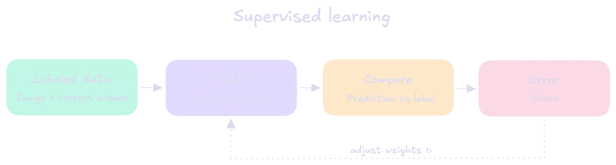
Supervised learning

Supervised learning is a type of machine learning where a model learns from labeled examples.

Each training example includes:

• an input (data)
• the correct output (label)

The model’s job is to learn the relationship between inputs and outputs so it can predict the correct output for new, unseen inputs.

Example: If you show a model many emails labeled “spam” or “not spam,” it learns patterns and can then classify new emails.

More resources

He also recommended these videos:

• Neural Networks explained
• The Dark Matter of AI [Mechanistic Interpretability]. This one felt a bit too advanced for me yet.

Tools

We use a public image dataset from Kaggle:

The dataset is structured in a simple folder format, where each class has its own directory. This makes it compatible with PyTorch’s ImageFolder, which automatically assigns labels based on folder names.

Our dataset hierarchy looks like:

data/
|-- test/
|   |-- chihuahua/
|   `-- muffin/
`-- train/
    |-- chihuahua/
    `-- muffin/

This structure separates training and testing data, allowing us to train the model on one set of images and evaluate it on unseen examples.

Tools used:

• Python
• VS Code IDE
• Jupyter Notebook Plugin for VSCode

The project uses the following dependencies, stored in requirements.txt:

• PyTorch (model building and training)
• Torchvision (image loading and transformations)
• Pillow (image file handling)
• Matplotlib (visualization)

torch==2.12.0
torchvision==0.27.0
matplotlib==3.10.9
pillow==12.2.0

To install the dependencies, we first create a Python virtual environment. This isolates the project so that its packages do not interfere with other Python installations on the system.

python -m venv venv
source venv/bin/activate
pip install -r requirements.txt

Let’s build

If you wish to access the notebook directly, here is my GitHub repository.

First we create a notebook.ipynb file.

We import PyTorch here to confirm the environment is set up correctly before going further.

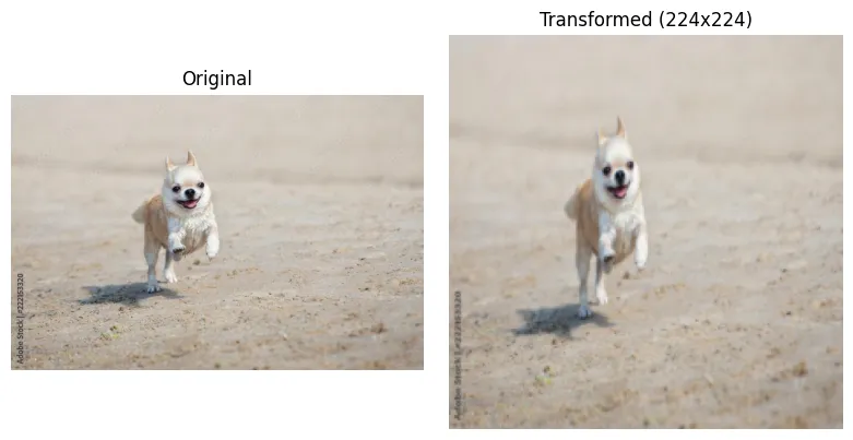
import torch

We prepare an image so it can be used as input for a neural network. Machine learning models cannot work directly with raw image files, so the image must first be converted into a numerical format they can process.

The image is resized to 224x224 because most neural networks require inputs of a fixed size. Without this step, images of different dimensions would not be compatible with the model.

Next, the pixel values are scaled to a range between 0 and 1 and converted into floating-point numbers. This makes the data easier and more stable for the model to learn from, since very large integer values (0-255) can slow down or destabilize training.

import matplotlib.pyplot as plt
import torchvision.transforms.v2 as transforms
import torch

from pathlib import Path
from typing import cast
from PIL import Image

PATH: Path = Path("./data/test/chihuahua/img_4_568.jpg")

img: Image.Image = Image.open(PATH).convert("RGB")

transform: transforms.Compose = transforms.Compose([
    transforms.Resize((224, 224)),
    transforms.ToImage(),
    transforms.ToDtype(torch.float32, scale=True),
])

img_tensor: torch.Tensor = cast(torch.Tensor, transform(img))

_, (ax1, ax2) = plt.subplots(1, 2, figsize=(8, 4))

ax1.imshow(img)
ax1.set_title("Original")
ax1.axis("off")

ax2.imshow(img_tensor.permute(1, 2, 0).numpy())
ax2.set_title("Transformed (224x224)")
ax2.axis("off")

plt.tight_layout()
plt.show()

Output:

We create training and testing datasets so the model can learn from one set of images and be evaluated on another it has not seen before. This separation is important because it lets us measure how well the model generalizes to new data instead of just memorizing the training images.

We use ImageFolder, which automatically reads images from folders where each class has its own directory. This makes it easy to assign labels based on folder names without manually labeling each image.

We apply the same transformations as before to ensure all images have the same size and format, and that pixel values are scaled between 0 and 1. This consistency is necessary so the model receives data in a uniform structure during both training and testing.

Finally, we print class_to_idx to see how class names (folder names) are mapped to numeric labels, which is what the model actually uses internally.

from torchvision import datasets
from torchvision.datasets import ImageFolder

transform: transforms.Compose = transforms.Compose([
    transforms.Resize((224, 224)),
    transforms.ToTensor(),
    transforms.ToDtype(torch.float32, scale=True),
])

train_dataset: ImageFolder = datasets.ImageFolder(
    root="./data/train",
    transform=transform,
)

test_dataset: ImageFolder = datasets.ImageFolder(
    root="./data/test",
    transform=transform,
)

class_to_idx: dict[str, int] = train_dataset.class_to_idx
print(class_to_idx)

Output:

{'chihuahua': 0, 'muffin': 1}

We create data loaders to feed images into the model in small groups called batches. Neural networks do not process one image at a time efficiently, so batching helps speed up training and makes better use of memory.

We set batch_size=32, which means the model will process 32 images at once before updating its weights. This improves training stability compared to processing single images.

We shuffle the training data so the model sees images in a different order each epoch, which helps prevent it from learning patterns based on the order of the data. We do not shuffle the test data because we want consistent evaluation results.

Finally, we load one batch from the training loader to check that everything works correctly. The image tensor shape shows 32 images with 3 color channels and 224x224 size, and the label tensor shows one label per image.

from torch.utils.data import DataLoader

train_loader: DataLoader[tuple[torch.Tensor, torch.Tensor]] = DataLoader(
    train_dataset,
    batch_size=32,
    shuffle=True,
)

test_loader: DataLoader[tuple[torch.Tensor, torch.Tensor]] = DataLoader(
    test_dataset,
    batch_size=32,
    shuffle=False,
)

images: torch.Tensor
labels: torch.Tensor
images, labels = next(iter(train_loader))

print(images.shape)
print(labels.shape)
print(labels)

Output:

torch.Size([32, 3, 224, 224])
torch.Size([32])
tensor([0, 0, 0, 0, 1, 1, 0, 0, 0, 1, 0, 1, 0, 0, 0, 1, 1, 0, 0, 0, 0, 0, 1, 0,
        0, 0, 0, 0, 0, 1, 1, 1])

We define a convolutional neural network (CNN) to learn patterns in images and classify them into two categories. The convolution layers act as feature extractors, detecting simple patterns like edges and textures first, then combining them into more complex features. Pooling layers reduce the spatial size of the image, which makes the model more efficient and helps it focus on the most important information.

After feature extraction, we flatten the data and pass it through fully connected layers, which act like a decision-maker. These layers take the extracted features and learn how they relate to the final classes. The last layer outputs two values, one for each class, which the model uses to make a prediction.

import torch.nn as nn
import torch

class SnifferCNN(nn.Module):
    def __init__(self) -> None:
        super().__init__()

        self.conv_layers = nn.Sequential(
            nn.Conv2d(in_channels=3, out_channels=16, kernel_size=3, padding=1),
            nn.ReLU(),
            nn.MaxPool2d(2),
            nn.Conv2d(in_channels=16, out_channels=32, kernel_size=3, padding=1),
            nn.ReLU(),
            nn.MaxPool2d(2),
        )

        self.fc_layers = nn.Sequential(
            nn.Flatten(),
            nn.Linear(32 * 56 * 56, 128),
            nn.ReLU(),
            nn.Linear(128, 2),
        )

    def forward(self, x: torch.Tensor) -> torch.Tensor:
        x = self.conv_layers(x)
        x = self.fc_layers(x)
        return x

We create the model and move it to the CPU so it is ready to process data. Printing the model shows its full structure, including all layers and their order. This helps us verify that the network was built correctly and understand how input data flows through it from convolution layers to the final classification output.

device: torch.device = torch.device("cpu")
model: SnifferCNN = SnifferCNN().to(device)
print(model)

Output:

SnifferCNN(
  (conv_layers): Sequential(
    (0): Conv2d(3, 16, kernel_size=(3, 3), stride=(1, 1), padding=(1, 1))
    (1): ReLU()
    (2): MaxPool2d(kernel_size=2, stride=2, padding=0, dilation=1, ceil_mode=False)
    (3): Conv2d(16, 32, kernel_size=(3, 3), stride=(1, 1), padding=(1, 1))
    (4): ReLU()
    (5): MaxPool2d(kernel_size=2, stride=2, padding=0, dilation=1, ceil_mode=False)
  )
  (fc_layers): Sequential(
    (0): Flatten(start_dim=1, end_dim=-1)
    (1): Linear(in_features=100352, out_features=128, bias=True)
    (2): ReLU()
    (3): Linear(in_features=128, out_features=2, bias=True)
  )
)

We define the loss function and the optimizer, which are two key parts of training a neural network.

The loss function measures how wrong the model’s predictions are compared to the true labels. Here we use CrossEntropyLoss, which is commonly used for classification problems (like deciding which class an image belongs to).

The optimizer controls how the model learns from that error. We use Adam, which updates the model’s parameters step by step to reduce the loss over time.

The learning rate (lr=0.001) controls the size of each update step:

• If it is too high, the model changes too aggressively and may miss the best solution.
• If it is too low, learning becomes very slow.

Together, the loss function and optimizer define how the model improves during training.

import torch.optim as optim

loss_function: nn.CrossEntropyLoss = nn.CrossEntropyLoss()
optimizer: optim.Adam = optim.Adam(
    model.parameters(),
    lr=0.001,
)

We train the model by showing it many batches of images and gradually adjusting its internal parameters to reduce errors. Each epoch means one full pass through the training dataset.

For each batch, we send the images through the model to get predictions, then compare those predictions to the correct labels using the loss function. This tells us how wrong the model is.

We then reset previous gradients, compute new gradients using backward(), and update the model using the optimizer. This is the step where the model actually learns by slightly adjusting its weights.

At the end of each epoch, we compute the average loss. A decreasing loss over time indicates that the model is improving its predictions.

epochs: int = 5

epoch: int
for epoch in range(epochs):
    model.train()
    total_loss: float = 0.0

    batch_images: torch.Tensor
    batch_labels: torch.Tensor
    for batch_images, batch_labels in train_loader:
        batch_images = batch_images.to(device)
        batch_labels = batch_labels.to(device)

        outputs: torch.Tensor = model(batch_images)
        loss: torch.Tensor = loss_function(outputs, batch_labels)

        optimizer.zero_grad()
        loss.backward()
        optimizer.step()

        total_loss += loss.item()

    print(f"Epoch {epoch + 1}, Loss: {total_loss / len(train_loader):.4f}")

Output:

Epoch 1, Loss: 0.6052
Epoch 2, Loss: 0.3601
Epoch 3, Loss: 0.2964
Epoch 4, Loss: 0.2346
Epoch 5, Loss: 0.1701

We test the model by switching it into evaluation mode so it behaves correctly during inference (for example, disabling training-specific behavior like dropout if it existed).

We take a single image from the test dataset and prepare it in the same format the model expects. Since the model processes batches, we add an extra dimension so the image becomes a batch of size 1.

We then run the image through the model without tracking gradients, because we are not training anymore. The model outputs scores for each class, and we select the class with the highest score as the prediction.

Finally, we compare the predicted label with the true label and display the image along with both values so we can visually check whether the model is performing correctly.

model.eval()

image: torch.Tensor
label: int
image, label = test_dataset[0]

image_input: torch.Tensor = image.unsqueeze(0).to(device)

with torch.no_grad():
    output: torch.Tensor = model(image_input)
    predicted: torch.Tensor
    _, predicted = torch.max(output, 1)

true_class: str = test_dataset.classes[label]
predicted_class: str = test_dataset.classes[predicted.item()]

print("True label:", true_class)
print("Predicted:", predicted_class)

title: str = f"True: {true_class} | Pred: {predicted_class}"

plt.imshow(image.permute(1, 2, 0).numpy())
plt.title(title)
plt.axis("off")
plt.show()

Output:

True label: chihuahua
Predicted: chihuahua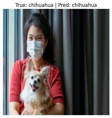

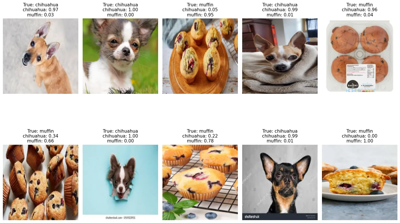
We evaluate the model on multiple random test images to get a better sense of its behavior instead of looking at just one prediction.

We first switch the model to evaluation mode so it behaves consistently during inference. Then we randomly select 10 images from the test dataset to avoid bias and to see varied examples.

For each image, we prepare it in the correct format by adding a batch dimension and passing it through the model without computing gradients. The model outputs raw scores, which we convert into probabilities using softmax so we can interpret them as confidence levels for each class.

We then display each image along with its true label and the model’s predicted probability for every class. This makes it easier to see not only whether the model is correct, but also how confident it is in its predictions.

model.eval()

indices: list[int] = random.sample(range(len(test_dataset)), 10)

plt.figure(figsize=(14, 10))

i: int
idx: int
for i, idx in enumerate(indices):
    image: torch.Tensor
    label: int
    image, label = test_dataset[idx]

    input_tensor: torch.Tensor = image.unsqueeze(0).to(device)

    with torch.no_grad():
        output: torch.Tensor = model(input_tensor)
        probabilities: torch.Tensor = F.softmax(output, dim=1)[0]

    prob_text: str = "\n".join(
        f"{name}: {probabilities[j].item():.2f}"
        for j, name in enumerate(test_dataset.classes)
    )

    true_class: str = test_dataset.classes[label]

    plt.subplot(2, 5, i + 1)
    plt.imshow(image.permute(1, 2, 0).numpy())
    plt.title(f"True: {true_class}\n{prob_text}", fontsize=8)
    plt.axis("off")

plt.tight_layout()
plt.show()

Output:

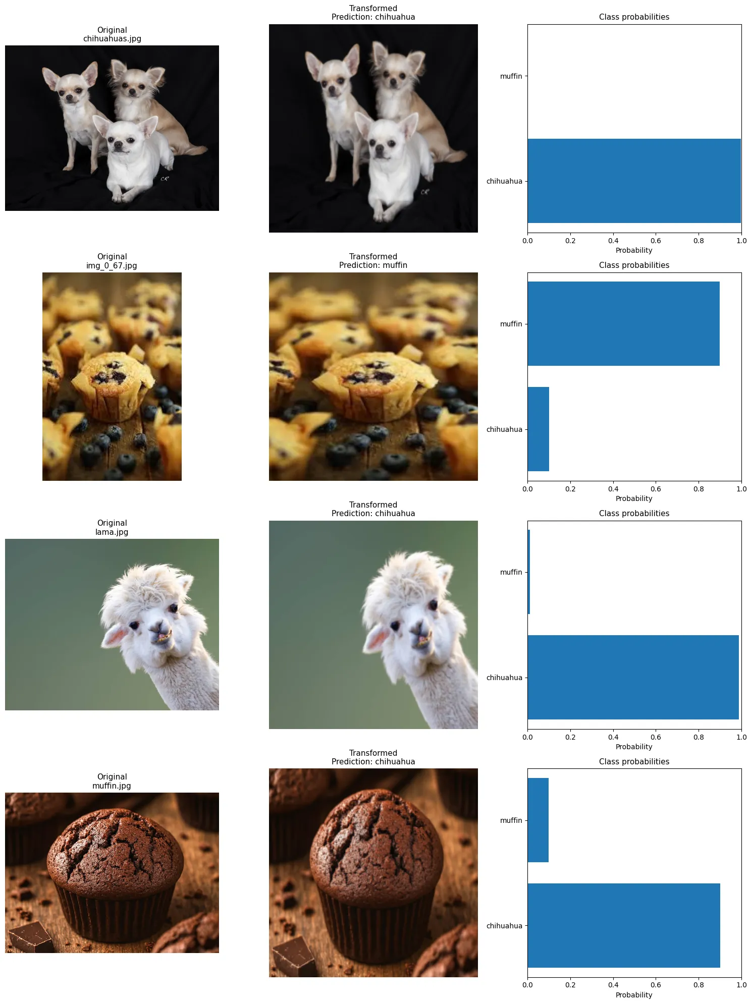
We use this code to test the model on completely new images and understand how it behaves on real inputs outside the dataset.

We first collect all images from a folder and load the trained model in evaluation mode so predictions are consistent. Each image is preprocessed using the same transformations as during training so the model receives data in the correct format.

For each image, we run inference to get both the predicted class and the probability for each possible class. These probabilities come from applying softmax, which converts raw model scores into values between 0 and 1 that sum to 1.

We then visualize three things side by side: the original image, the transformed version that the model actually sees, and a bar chart showing the model’s confidence for each class. This helps us understand not only what the model predicts, but also how certain it is.

import torch.nn.functional as F

img_paths: list[Path] = sorted(Path("./data/others").glob("*.jpg"))
img_paths: list[Path] = sorted(
    p for ext in ("*.jpg", "*.jpeg", "*.png")
    for p in Path("./data/others").glob(ext)
)

model.eval()

n_cols: int = 3
n_rows: int = len(img_paths)
plt.figure(figsize=(15, 5 * n_rows))

img_path: Path
for i, img_path in enumerate(img_paths):
    image: Image.Image = Image.open(img_path).convert("RGB")
    image_tensor: torch.Tensor = cast(torch.Tensor, transform(image))

    input_tensor: torch.Tensor = image_tensor.unsqueeze(0).to(device)

    with torch.no_grad():
        output: torch.Tensor = model(input_tensor)
        predicted: torch.Tensor
        _, predicted = torch.max(output, 1)
        probabilities: torch.Tensor = F.softmax(output, dim=1)

    class_name: str = test_dataset.classes[predicted.item()]

    probs: list[float] = [p.item() for p in probabilities[0]]

    # left: original image
    plt.subplot(n_rows, n_cols, i * n_cols + 1)
    plt.imshow(image)
    plt.title(f"Original\n{img_path.name}", fontsize=9)
    plt.axis("off")

    # middle: transformed image (denormalized for display)
    plt.subplot(n_rows, n_cols, i * n_cols + 2)
    plt.imshow(image_tensor.permute(1, 2, 0).numpy())
    plt.title(f"Transformed\nPrediction: {class_name}", fontsize=9)
    plt.axis("off")

    # right: probability bar chart
    plt.subplot(n_rows, n_cols, i * n_cols + 3)
    plt.barh(test_dataset.classes, probs)
    plt.xlim(0, 1)
    plt.xlabel("Probability")
    plt.title("Class probabilities", fontsize=9)

plt.tight_layout()
plt.show()

Output:

We evaluate the model on the test dataset to measure how well it generalizes to unseen data. We switch the model to evaluation mode so it behaves correctly during inference, and we disable gradient tracking because no learning happens during testing.

We loop through the test data in batches, pass each batch through the model, and take the class with the highest score as the prediction. We compare predictions with the true labels and keep a running count of correct predictions and total samples.

We then compute accuracy by dividing correct predictions by the total number of samples. This gives a single metric that summarizes model performance on the test set.

Finally, we also print the total number of trainable parameters in the model to understand its size and complexity.

model.eval()

correct: int = 0
total: int = 0

with torch.no_grad():
    batch_images: torch.Tensor
    batch_labels: torch.Tensor
    for batch_images, batch_labels in test_loader:
        batch_images = batch_images.to(device)
        batch_labels = batch_labels.to(device)

        outputs: torch.Tensor = model(batch_images)

        predicted: torch.Tensor
        _, predicted = torch.max(outputs, 1)

        total += batch_labels.size(0)
        correct += int((predicted == batch_labels).sum().item())

accuracy: float = correct / total
print(f"Test Accuracy: {accuracy:.4f}")

total_params: int = sum(p.numel() for p in model.parameters())
print(f"Total parameters: {total_params:,}")

Output:

Test Accuracy: 0.8446
Total parameters: 12,850,530

The test accuracy of 0.8446 means the model correctly classified about 84.46% of the images in the test dataset. This gives an estimate of how well the model generalizes to new, unseen data. The remaining errors show cases where the model made incorrect predictions, which can happen due to similar-looking classes, limited training data, or model limitations.

The model has 12,850,530 parameters, which represents the number of learnable weights and biases inside the network. This value reflects the model’s capacity: more parameters allow the model to learn more complex patterns, but also increase memory usage and the risk of overfitting if the dataset is too small.

For comparison:

This model: ~13 million parameters Small language models (like BERT-base): ~110 million parameters (about 8x bigger) Large language models (like GPT-3): ~175 billion parameters (over 10,000x bigger) Very large modern models: even larger, but exact sizes are not always public

So this image model is relatively small compared to modern language models, but still large enough to learn useful visual patterns.

Going further

There are several practical ways to improve this image model and deepen my understanding of how larger models work.

• more parameters (animals): Make the model bigger (more layers or filters). This can help it learn more detailed patterns, like differences between similar animals, but it also needs more data.
• add normalization: Standardize the input data so values are in a consistent range. This usually makes training more stable and faster.
• larger dataset (fine tuning): Train on more images or start from a model that was already trained on a large dataset. Then adjust it for your specific task, similar to how LLMs are adapted for different uses.
• Data augmentation: Create variations of training images (flip, rotate, crop, color change). This helps the model generalize better and reduces overfitting.
• More training epochs + monitoring loss: Train longer while tracking validation loss to avoid stopping too early or overfitting.
• Better model architecture: Replace the simple CNN with a pretrained model like ResNet or EfficientNet. These are much stronger and already trained on large datasets.
• Learning rate tuning: Try different learning rates. Small changes can significantly affect performance.
• Validation set: Split test data into validation + test. Validation is used during training to tune settings, test is only for final evaluation.

Thoughts

This exercise was done in an afternoon. I am happy I did it, it helped me gain vocabulary, understand what an example setup looks like, and get a first practical sense of how a model is created and trained.

I feel like there is still a lot more to understand because there are many different types of neural network models, and PyTorch does most of the heavy lifting. I have yet to truly understand the maths behind the library’s functions, which is probably the next important step.